Personalized Medicine: Redefining Cancer Treatment /Predict the effect of Genetic Variants to enable

Once sequenced, a cancer tumour can have thousands of genetic mutations. But the challenge is distinguishing the mutations that contribute to tumor growth (drivers) from the neutral mutations (passengers).

Currently this interpretation of genetic mutations is being done manually. This is a very time-consuming task where a clinical pathologist has to manually review and classify every single genetic mutation based on evidence from text-based clinical literature.

For this competition Memorial Sloan Kettering Cancer Center (MSKCC) is making available an expert-annotated knowledge base where world-class researchers and oncologists have manually annotated thousands of mutations.

In this competition you will develop algorithms to classify genetic mutations based on clinical evidence (text).

There are nine different classes a genetic mutation can be classified on.

This is not a trivial task since interpreting clinical evidence is very challenging even for human specialists. Therefore, modeling the clinical evidence (text) will be critical for the success of your approach.

Both, training and test, data sets are provided via two different files. One (training/test_variants) provides the information about the genetic mutations, whereas the other (training/test_text) provides the clinical evidence (text) that our human experts used to classify the genetic mutations. Both are linked via the ID field.

Therefore the genetic mutation (row) with ID=15 in the file training_variants, was classified using the clinical evidence (text) from the row with ID=15 in the file training_text

File descriptions

1.0     Problem Definition

As technology progresses, advancements in precision medicine occur at an increased rate. Precision medicine is the idea of specifying treatment to patients based on their genetic make up. Currently, people with the same disease would be given the same treatment. Due to different genetic makeups, however, each patient may respond differently to the treatment since their genetics are not taken into account (Schork, 2015). Precision medicine hopes to solve this problem. By considering the patient’s genetics, doctors can have a better understanding of how they may react to the treatment and recommend an alternative treatment. In regard to cancer, precision medicine is very beneficial. There are many types of cancers that are all differentiated in terms of the treatment that is necessary for each type. Patients with the same type of cancer and who are at the same stage would typically be given the same treatment. However, each patient may have different mutations in their tumour which may cause them to respond differently to the treatment (Van’t Veer & Bernards, 2008).

Analyzing mutations in the sequence of a tumour cell can provide critical information as to how the tumour will behave. All cancerous tumours are malignant, however they have thousands of different mutations that impact the way that they behave. Two people with the same tumour may have different mutations of that tumour that would impact its behaviour. Certain mutations are more detrimental than others, in that they drive the tumour’s growth. These types of mutations are referred to as drivers and they provide a selective growth advantage on the tumour, thus promoting cancer development. The other neutral mutations are referred to as passengers and have no effect on the growth of the tumour (Bozic, et al., 2010). Knowing whether a mutation will contribute to the growth of the tumour or not is highly beneficial, although this is difficult to determine manually. There is a large amount of research available regarding the many variants that are found in cancer tumour genes and whether or not a specific variant contributes to the growth of the tumour. Although this information is readily available, it is a difficult task to aggregate the data from literature and classify the thousands of mutations manually. We need a way to automate the process of differentiating between a passenger and a driver mutation. With this knowledge, targeted drugs can be created that work for specific mutations of a certain tumour. This is a step in the right direction for precision medicine, as patients will be able to receive the drug that will target the specific mutation in their tumour, instead of a general drug that would target that tumour as a whole. Patients with the same tumour but different mutations would each receive different drugs corresponding to the respective mutations.

There are many factors involved in determining if a mutation is a driver or passenger. These factors include the frequency of the mutation, type of mutation, the class of the mutation, as well as many other things (Carter, et al., 2009). Due to these variety of factors, it is quite difficult to say with certainty if a mutation is a driver or passenger. Determining if a mutation is a driver of the tumour’s growth takes many things into account and is out of scope for this project. Thus, for this project, the focus will be placed on defining the class of the mutation, which is a critical step in determining the likelihood of a mutation being a driver versus a passenger.

There are nine different classes that a mutation can fall under, although it is important to note that these are not official classes found in literature. The nine classes of a mutation are likely loss of function, likely gain of function, neutral, loss of function, likely neutral, inconclusive, gain of function, likely switch of function, and switch of function (Kaggle, 2017). The labels of each of the classes essentially describe the effect that the mutation will have on the gene. Knowing the class of a mutation can help indicate the likelihood of it being a driver or passenger. Based on these class definitions, it is likely that the mutation classes that are neutral are highly likely to be passengers and not drivers. The classes that do affect function have a higher likelihood of being a driver, although they can be passengers as well depending on other factors. Due to this, we cannot say with certainty that any mutation that falls under a class that affects function would be a driver.

In this project, we will build a model that will use the research already conducted by scientists to predict the class of a given gene mutation. Identifying the class of a mutation will help indicate the behaviour of the tumour. This can ultimately assist the development of precision medicine for cancer treatment.

2.0      Data Understanding

Before preprocessing the data, it is important to first analyze the raw data to find significant patterns and correlations to class. This will provide a basis for pre-processing the raw data.

2.1      Class Distribution

The bar charts compare class distribution in the training data and validation data. Both of the data sets have minority classes (3, 8, 9) and the class 7 is the highest. Although training data and validation data share a similar trend, there is no duplicate row among these two files. Nonetheless, to prevent our machine learning algorithms from poor performance, finding a proper way to balance our imbalanced data is an important task to tackle. 

2.2      Mutation Distribution

These three graphs compare the numbers of 17 mutation types. SNP mutation constitutes the most among the three datasets (Training/Testing/Validation). Based on its imbalanced distribut

ion, it inspired us to separate our data into SNP data and non-SNP data. By running and evaluating them separately, the machine learning algorithms would not be biased towards the majority class. The distribution is imbalanced in each of the datasets and initial we attempt to model using a training set of SNP mutations. In our final models however we incorporate the entire data set. In future work, a model could be built that has individual models trained on SNP mutations and others trained on Non-SNP mutations in order to account for all mutations that could be presented to the model.

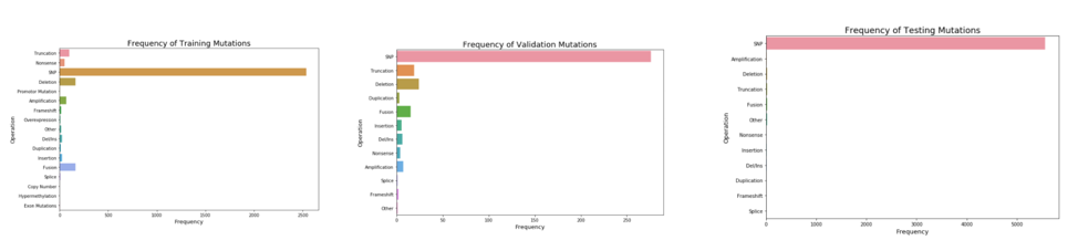
Figure 2.2 Mutation Distribution and Correlation to class

2.3      Genes Correlation to Class

The heatmap shows the correlation between Genes and Classes. This helps us understand how important the gene is in each class. There are four examples:

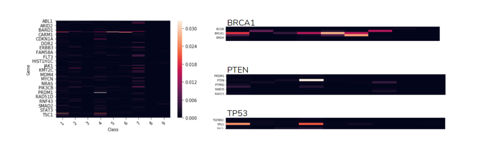
Figure 2.3 Genes Correlation to class

Figure 2.3 shows that gene “BRCA1” occurs almost in every class (top right), except of class 3,8,9. In contrast gene “PTEN” happens mostly in class 4 (middle right). Another highlight is how  gene “TP53” occurs in two specific classes, class 1 and 4 (bottom right). From Figure 2.3 , it shows that almost all types of genes happened in class 7. Therefore, we could assume that a great amount of the gene mutations are more likely to be class 7 (Gain-of-function).

2.4      Mutation Distribution Correlation to Class

The graphs in Figure 2.4 below shows the correlation between different mutation types and each class. Comparing the Unbalanced graph with Balanced one, the later one balanced the minority classes (3, 8, 9) and help us better visualize the distributions among minority classes. As expected SNP mutations comprises a large part in almost all the classes, compared to the other mutation types. We do see some variation in the distribution of SNP mutation between the 9 classes. It is expected that mutation type have some predictive power in the model.

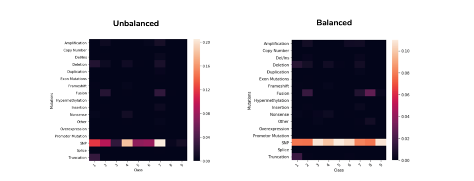
Figure 2.4 Mutation Distribution Correlation to class

2.5      Amino acid Distribution and Correlation to Class

The four graphs illustrated in Figure 2.5 show the correlation between the start amino-acid/end amino-acid (for the SNP mutation) and 9 classes. Although the unbalanced graphs are clearer for the differences, the balanced graphs are more proper to use since all the data in each class has all been normalized. After balancing the data, the SNP mutations that have the start amino-acid “R” occur frequently in class 9. Also, the ones that have the end amino-acid “R” happened much more frequently in class 8. 

Figure 2.5 Amino acid Distribution and Correlation to class

2.6      Mutation Location Correlation to Class

Figure 2.6 shows the correlation between SNP location bins and classes. From these two heatmaps we could say that most of the SNP location happened below 500. Also, for the class 4, SNP mutation happens mostly with location 0~250. After balancing the data, we could tell that in the class 9, SNP mutation happens mostly in location bins (0~250) and (500~750). 

Figure 2.6 Mutation Location Correlation to Class

2.7      Top TF-IDF Scores Words Correlation to Class

The graph depicted in Figure 2.7 illustrates top 10 TF-IDF scores for training text data. From bottom up, the bigger the block is, the more important the word is. By extracting these valuable words in each class, we can potentially use them to predict class. Also, by analyzing the duplication between these highest TFIDF words in each class, there are a couple classes share the same words. For instance, Class2,7 : 7 words in common /Class 1,4 : 6 words in common 

/Class 3,5 : 3 words in common /Class 8,9 : 2 words in common. These similarities might affect the performance of machine learning model.

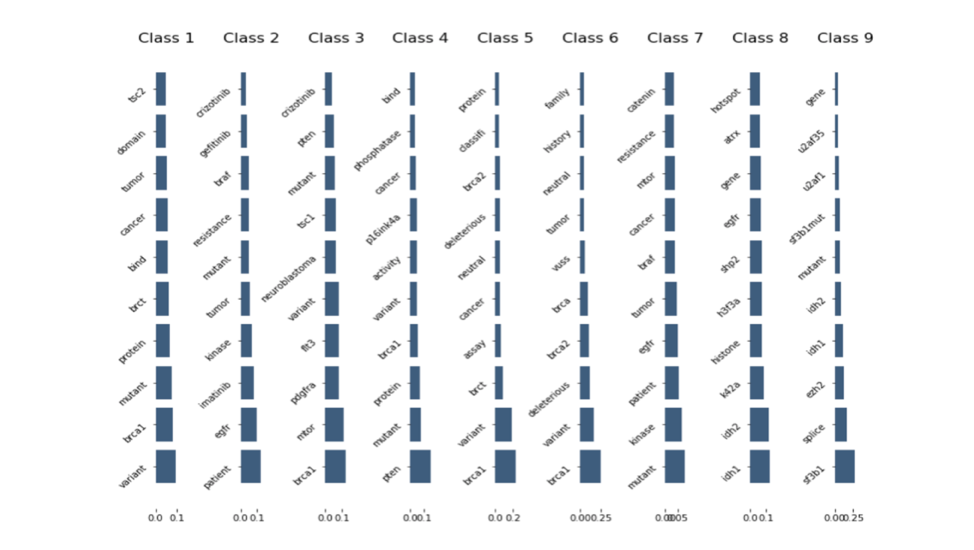
Figure 2.7 Top TF-IDF Scores Words Correlation to Class

2.8      Driver/Passenger Distribution Correlation to Class

Figure 2.8 shows whether the words “driver” and “passenger” appear in their corresponding text files in 9 classes. If it does appear, it would return 1. If it doesn’t, it would return 0. Before balancing the data, we could tell that “driver” appears often in class 7 and “passenger” almost doesn't occur in class 7. Thus, we could assume class 7 is more likely to be a driver. After balancing the data, “passenger” barely occurs in all classes. Therefore, by observing the frequency of “driver” happened in each class, we could predict their confidence of probability being a driver.

Figure 2.8 Driver/Passenger Distribution Correlation to Class

3.0      Challenges

3.1      Imbalanced Data

As shown in Figure 2.1, there is a severe imbalance of records available across the nine classes. Class 7 is very highly represented while there are almost no records for class 8 and 9. Imbalanced data will throw off the model and it will have a hard time predicting these more rare classes, although it will still maintain a high accuracy. This may cause underfitting for the respective classes since there is not enough data available to get any meaningful information.

3.2      Categorical Attributes

In order to use specific models, all attributes must be numerical values since the models cannot work with categorical values. Our data frame currently has attributes that are categorical values, and thus will need to be changed to become numerical values. This is essential for the model to run.

4.0      Methodology

A text mining approach will be used to create the model, as the basis of the model involves identifying meaning and patterns from the text. This model will be built using the given files: “training_variants.txt” and “training_text.txt”. The training text file is a file that contains a collection of research articles that discuss genes and their variations. These are the articles that were used to classify the various genetic mutations. The training variants file is another text file that contains the gene ID, variant, and the class that corresponds to the articles in “training_text.txt”. This data will be separated into both a training set and a testing set. Both these files will be used simultaneously to train the model. Once the model is built, it will be able to output the predicted class of the mutation of any given research article. The function and accuracy of this model will then be tested with the separated testing set.

4.1 Data Preparation

Before a model can be built based on the data given, it needs to first be pre-processed into clean data that can be used for accurate analysis. Raw data can contain anything from duplicates to missing values. In order to create a model that is accurately representative of the data, issues like missing data need to be dealt with to prevent any kind of bias or misrepresentation from the raw data.

In terms of text mining, specifically, there are several crucial pre-processing steps that are mandatory before moving on to the modelling of the data. These steps are text tokenizing, cleaning, and filtering. In addition to cleaning the data, new features can be generated based on the existing data. These new features will provide additional information and may have relevant correlations with mutation classes. All of the above steps will be completed using various libraries in python.

4.1.1     Cleaning Variants File

The focus is first put on cleaning the variants files “training_variants.txt”. The function var_clean takes a file var_file and opens it as a data frame using the Pandas library. It transforms all of the values in the “Variation” column to uppercase in order to standardize all the values. This is important since strings are case-sensitive and the lowercase version of the same word would typically be read as a completely different word by python. Once this is done, the function will move on to feature generation.

A new column “Mutations” is created. This column looks at the value in “Variation” and deduces the type of mutation it is, such as deletion, insertion, etc. The generation of this new feature is important as it extracts the specific type of mutation out of the variation. This way, multiple variations of the same mutation type will be considered the same. There is no need to consider them as different mutations.

Next, the columns “SNP Location”, “Start aa”, and “End aa” are created. These columns focus on the SNP mutations and extract the location of the SNP, the initial amino acid, and the final amino acid that it mutates to. For mutations that are not SNPs, the values in these columns are set to NaN. To simplify the data, we recognize that the location of each SNP is highly specific and can be analyzed as a range instead of specific numbers. SNP locations are thus chosen to be binned in bins of range 250 in a new column “SNP bins”.

Once the new features are all generated, both the “SNP Location” and “Variation” columns can be deleted, since these columns do not provide any additional information anymore. The function returns the cleaned data frame.

4.1.2    Cleaning Text Files

The function text_open takes a file text_file and opens it as a data frame. The text file is of the format where the ID is separated from the article by double pipes. text_open takes this into account and separates the file into a data frame based on the double pipes. When opening the file, we also specified that the encoding will be in UTF-8. This ensures proper encoding across the text attribute. Once the file is opened as a data frame, feature generation is done to create the attributes “Driver”, “Passenger”, and “Driver+Passenger”. The “Driver” and “Passenger” column contains information on whether the respective terms are found within the article. The “Driver+Passenger” column contains information on whether both the terms “driver” and “passenger” are found in the article together.

4.1.3  Merging Variants and Text Data Frames

In order to simplify the analysis of the data, the variants data and the text data will be merged together into one data frame. This way, visualization of patterns and analysis of the data will be much more convenient. Both data frames can be merged on “ID”. The function text_var takes in the two data frames var_df and text_df, merges them into one, and returns the final, merged data frame. In addition to merging the two data frames, it also deletes any rows where there is a missing value in the “Text” column. This is done since if there is no article in the record, no information can be gathered from it and the record is useless. 

Once the data frames are merged, duplicate records can be deleted from the data frame. This step was held off until after the data frames were merged in order to remove any redundancy. If duplicates were deleted before the data frames had merged, the deletion of duplicates would have had to happen twice for each data frame. The function remove_dups takes the data frame df and removes any records that contain the exact same value in each of the columns, excluding the ID column since those are unique values. The following is what the resulting data frame will look like:

📷

4.2     Removing Outliers

After further analysis of the value counts of the resulting data frame, there seemed to be outliers in the “End aa” column. This column should only contain the possible amino acids, however there appeared a “7” and a “5”, which cannot be scientifically accurate for a SNP mutation and thus must be an error in the data. Since this is the case, it is acceptable to drop the entire record from the data frame.

4.3 Text Tokenizing and Filtering

Now that the data is cleaned, the “Text” column needs to be tokenized and filtered into significant words. Ideally, the resulting tokens should provide meaning and be correlated with predicting mutation class. The method used to complete this is TF-IDF. This method takes the product of term frequency and inverse document frequency. This method was chosen because it selects for valuable words. These are words that are rare in the majority of records but common in a small subset of them. If the TF-IDF score of a word is high, it means that the given word is common among a small portion of the records, thus proving to be a valuable word that may provide meaning for the model. 

With narrowing down valuable words using TF-IDF, it is also beneficial to remove any stopwords from the tokens. These are filler words that do not provide any significant meaning. In addition to the available list of stopwords found online, we have added extra stopwords that are relevant to the research articles. These include words such as “figure”, “analyze”, etc. As well, we also remove any number strings, since numbers do not provide any meaningful information to the model. Additionally, tokens that are less than 3 characters in length are removed. 

Before TF-IDF vectorization occurs, the tokens are lemmatized. This was chosen over stemming due to time restraints. Stemming required much more time to run in comparison to lemmatizing. The difference between stemming and lemmatization is that lemmatization results in tokens that are real words, while stemmed tokens may not be real words. As a result, lemmatization treats words like “active” and “activate” as different, though they have the same meaning. 

Following vectorization the TF-IDF array was converted into a pandas DataFrame and merged with the training dataset. The Text feature in the training dataset is removed prior to the merge. 

4.4      Dummy Encoding

As stated in section 3.2, the models to be used require numerical values. Thus, all numerical values must be converted to categorical values. This can be done through dummy encoding. The categorical attributes currently in the data frame are Mutation, Start aa, and End aa. For each value in these attributes, a separate column was created where a value of 1 is assigned if the attribute is found in the record and a zero is assigned otherwise.

4.5      Split and Over Sample Data

Now that the data is cleaned and ready to be modelled, it is split into both a training set and a testing set. The training set consists of 67% of the records in the data frame while the testing set consists of the other 33%. The training set is what will be used to train the model, and the test set will be used on the completed model in order to test its accuracy.

Once the data is split, it needs to be balanced across the classes. Figure 2.1 illustrates the number of records available for each of the nine classes. It is clear in the figure that classes are severely underrepresented and there is an imbalance in the data. In order to fix this issue, random oversampling will be done on the “Class” attribute. The RandomOverSampler() function from the imbalanced-learn library is used to complete this. Once this is done, a plot is created depicting the resulting number of records for each class. This visualization is executed in order to confirm that the oversampling worked correctly.

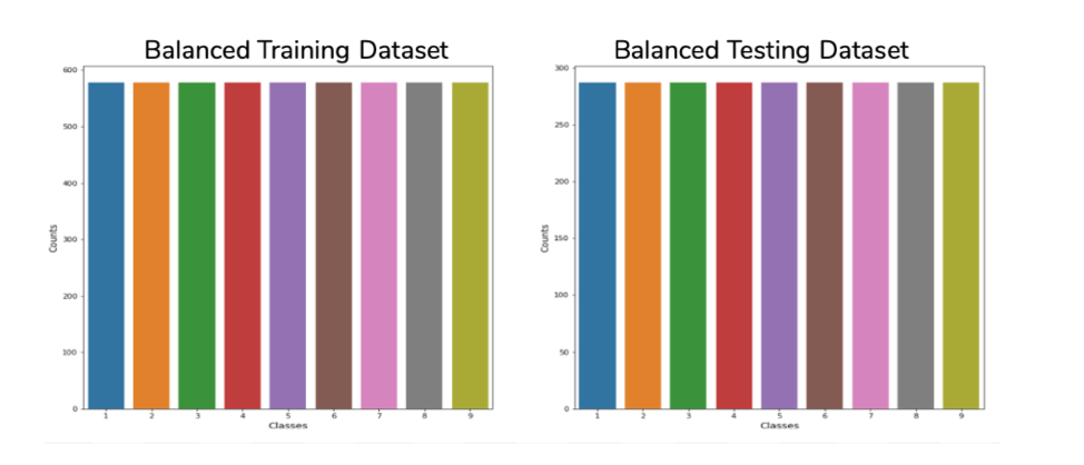
Figure 4.5: Bar plot depicting the number of records per class count. In the split training and testing  dataset.

As shown in Figure 4.5, it is clear that the oversampling was successful and the data is now balanced across the nine classes. The same balancing is done for the testing data set as well.

5.0      Evaluation

5.1      Individual Model Evaluation

Now that the data is preprocessed and prepared, we can begin modelling and evaluating. Six individual models will be tested in order to evaluate the individual accuracies. The six models to be tested are random forest, decision tree, SVC, K-nearest neighbour, gradient boosting, and logistic regression. The following shows the individual models and their testing accuracy:

Random Forest : 41%

Decision Tree: 100%

SVC: 100%

K Nearest Neighbor: 55%

Gradient Boosting: 100%

Logistic Regression: 59%

Comparing the accuracy of random forest and decision tree, it turns out that aggregated/ensemble models (random forest) are not universally better than their single counterparts (decision tree).

After testing each individual model’s accuracy, it helps to determine which models are more suitable to use. For instance, to create an ensemble or stacked model, we could choose which models to put in based on the accuracy of models. The models chosen to be used for the stacked model should be above a 50% accuracy. Based on the accuracy of the six models, we decided to use K-nearest neighbour, gradient boosting, and logistic regression in a stacked model.

5.2      Stacked Model Evaluation

Each model is trained on the training set and makes a prediction on the test data. The results of each model's predictions are stored in a pandas data frame. The confusion matrices for each of the three models being used in the stacked model are as follows:

The data used for the K-nearest neighbour model is all mutation types, while logistic regression and gradient boosting use the mutation, start & end amino acid, as well as the TF-IDF values. When evaluated, the stacked model gives an accuracy score of 56%. The following is the confusion matrix of the stacked model:

The Matthews correlation coefficient is 0.52, which is a decent score but could be better. The mean precision is 50%, the mean recall is 56%, and the mean f1 score is 0.52. As shown, the stacked model does not improve the accuracy of the model significantly. A possible improvement to this model can be to use different models within the stacked model. For example, one vs. rest and neural networks were not tested due to time constraints. These models may prove to have a higher accuracy and can thus be used in the stacked model to increase accuracy. As well, the issue of imbalanced mutations may be causing the model to be faulty. If we had a separate model for non-SNP mutations, we may see an increase in accuracy. 

5.3      Ensemble Model Evaluation

In order to further test our model and obtain a higher accuracy, the same three models were used in an ensemble. The confusion matrix for the ensemble model is shown as follows:

The accuracy score of this ensemble model is 77%, a 21% increase from the stacked model. The Matthews correlation coefficient is 0.75 which is ideal since the closer to 1, the better the model is. The mean precision is 79%, the mean recall is 77%, and the mean F1 score is 0.77.

Aside: It is important to note that after completion of the stacked and ensemble models, it was discovered that the testing set being used included class information. As a result, the accuracy of the models was inflated and is not an accurate representation of the model’s true capabilities. When tested with the proper testing data, the ensemble gave an accuracy of 45% and the stacked model gave an accuracy of 25%. Due to time constraints, it was not feasible to tune the parameters to fix these accuracy errors, as we used default parameters. We include code for each of the model types for the incorrect and corrected datasets. 

6.0      Conclusion

Using a text mining approach, a machine learning model was developed that would be able to extract information from research articles to predict the class of the mutation. The final ensemble model developed is able to predict mutation class with an overall accuracy of 45%. The machine learning model used was an ensemble, which contained k-nearest neighbour, gradient boosting, and logistic regression. The overall model uses the attributes mutation type, start amino acid, end amino acid, TF-IDF values, as well as the presence of “driver” in text in order to predict the mutation class. This model can provide the means to do further research into applying this model to precision medicine. 

7.0      Future Work

Although a model was created to predict mutation classes, there is much more refinement and further steps that can be taken in order to further improve our solution. Now that a trained model has been developed, it is important to test the model using separate data, such as the stage_2 data. This is essential in determining the true accuracy of the model.

7.1      Amino Acid Mutation Distance Mapping

For SNP mutations, the change from one amino acid to another can either be highly detrimental to the protein or not affect the protein at all. Amino acids all greatly differ from each other in terms of their physical and chemical properties. These differences are due to their side chains.  As a result, the various amino acid replacements are scored differently, where the scores reflect how severely the replacement will affect the protein. Typically, the less similar the amino acids are in terms of their physicochemical properties, the more negative their score will be. For example, a polar amino acid changing to a polar amino acid will not do a great deal to the function of the protein, however the same cannot be said if it changed to a nonpolar amino acid. Figure 7.1 shows the BLOSUM matrix representing the scores of the various amino acid substitutions. 

Figure 7.1: BLOSUM matrix depicting amino acid substitution scores.

In the future, a new feature can be generated in the data frame that reflects these substitution scores. This would give the model significant, additional information that will improve the accuracy of its predictions.

7.2      Improve Modeling

Due to time constraints, it was difficult to complete the process of refining our model. Since the final model’s accuracy is only 45%, improvement of the model should be done. In regards to balancing our data, we can try other methods to complete this task. One thing that can be done is to change the class weights. As well, instead of oversampling the data, SMOTE can be used to balance the classes. With SMOTE, there is less chance of overfitting and will prevent duplicates. SMOTE was originally not used out of fear of creating misclassified samples.

The algorithm parameters used can be tuned to better represent our data. Currently, the parameters used are the default parameters assigned by the python libraries. By setting parameters that are specified to the data, it will increase the likelihood of the model having a better accuracy. In order to do this, multiple parameter combinations will need to be tested to see which combination gives the highest accuracy. While GridSearchSVC provides a means of doing so it is  a time consuming process which is why this could not be completed at this point. 

In addition to fine tuning the algorithm parameters, the TF-IDF vectorization can also be polished. The max features are currently set to 1000, however this can be further pruned. The max_df and min_df can be set to specific numbers in order to cut out records that are not valuable. As well, lemmatization is used in the current model instead of stemming, even though stemming would provide more valuable tokens. As stated in section 4, stemming required quite a bit more time and was not feasible to complete. In the future with more time, stemming of the tokens can be done to narrow down the TF-IDF features.

7.3      Further Feature Generation

In order to extract more meaning from the articles, a significant step that could be taken would be to focus mainly on sentences that contain the gene of interest. This will exclude much of the extra information from the articles that are not involved in predicting mutation class. By focusing on these sentences solely, the resulting tokens that are generated will be more specified and ultimately improve the model’s accuracy.

7.4      Predicting Other Mutations

As noted in section 2, Figure 2.2 depicts the breakdown of the different mutations. The SNP mutations are very highly overrepresented in comparison to all the other types of mutations. As a result, the data available on the other mutations are not enough to come to accurate conclusions. A solution to this issue can be to separate the other mutations from the SNP mutations and model the data separately. By separating the SNP mutations and the other mutations and modelling them separately, we prevent any kind of bias that may arise out of the imbalanced data. 

7.5      Determining Driver & Passenger Mutations

As stated in section 4, the scope of this project only covers predicting the class of a tumour gene mutation. In the future, this model can be updated to include additional information that will help indicate the likelihood of a mutation being a driver or a passenger mutation. There are many factors that need to be considered in order to predict this information accurately. This information may or may not be present in the research articles found in the files, so additional research may be required in order to predict this information. External gene databases can be used to extract the necessary information.

8.0      Work Cited

Bozic, I., Antal, T., Ohtsuki, H., Carter, H., Kim, D., Chen, S., ... & Nowak, M. A. (2010). Accumulation of driver and passenger mutations during tumor progression. Proceedings of the National Academy of Sciences, 107(43), 18545-18550.

Kaggle. (2017). Personalized Medicine: Redefining Cancer Treatment. NIPS.

Schork, N. J. (2015). Personalized medicine: time for one-person trials. Nature News, 520(7549), 609.

Van't Veer, L. J., & Bernards, R. (2008). Enabling personalized cancer medicine through analysis of gene-expression patterns. Nature, 452(7187), 564.

Vitkup, D., Sander, C., & Church, G. (2003).The amino-acid mutational spectrum of human genetic disease. Genome Biol, 4(11).

*the link of the code we wrote : https://github.com/ChristineWeitw/Biomedical-datamining/blob/master/Good-Modelling-tfidf-sample-on-full-dataset-with-stacking%20(1).ipynb

*the data can be accessible through this Kaggle competition's link: https://www.kaggle.com/c/msk-redefining-cancer-treatment/data